

Debates about the ‘best’ way to invest never end.
So, we decided to put one idea to the test.
What would happen if you invested only when the market is undervalued, and sit out the expensive periods?
To find out, we ran a 10-year simulation (2015–2025) comparing a simple, timing-based strategy against a regular, continuous SIP.
The Setup
We looked at 2 approaches:
The Consistent SIP Investor: invests in the market every month, no matter what. For this, we used the Nifty 50 Index Fund.
The Market Timer: invests only when the market looks ‘undervalued’.
But how do you decide if the market is undervalued?
We used the Nifty 50’s P/E ratio as a guide: whenever it fell below a set level the market was considered undervalued.
We tested three different PE ratio cutoffs (15, 20, or 25) to see the results.
And what was the strategy?
If P/E was below the cutoff — the monthly investment went into the index fund.
If P/E was above the cutoff — the monthly investment was put in debt funds/FD/bonds that gave a steady 6% return per annum.
Whenever the P/E dipped back below the cutoff, all the debt fund/FD investments, along with that month’s investment, were moved into the index fund.
So to put it simply — invest in the index fund only when the market is undervalued, otherwise let your money sit in debt funds while you wait for the right time.
One important detail: whenever money is taken out from the debt funds, there are taxes that apply on the interest earned. (We used current tax rates for simplicity, though tax rules have changed over the years).
We ran this cycle over a 10-year period (120 months) from September 2015 to August 2025. The UTI Nifty 50 index fund represented the investments in the market.
What would the final portfolio look like if you followed this timing strategy versus just investing consistently in the index fund every month?
Which approach would have delivered better returns over a decade?
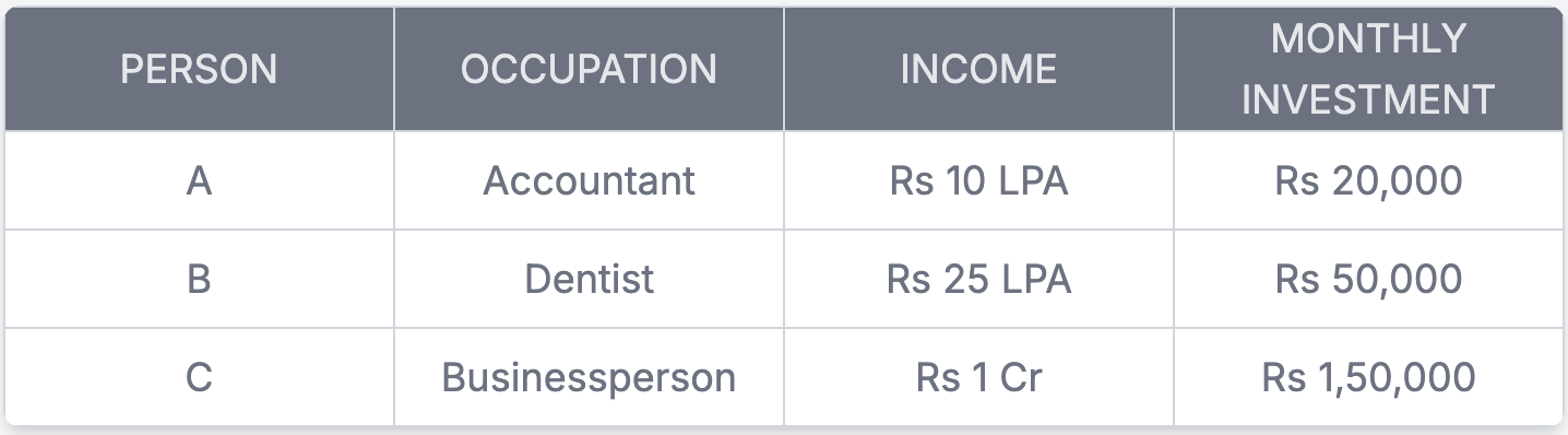
The People in Our Study
To make it relatable, we imagined 3 different people earning different incomes:
We ran this simulation using a Python program. If you want, you can check out the code below and try the experiment yourself.
Let’s start with the accountant, who invests Rs 20,000 every month.
If they keep investing in the index fund regardless of the market (SIP), their portfolio at the end of the 10-year period will look like this:
--- Final Results ---

Total Amount Invested: ₹0.24 crores or 24 lakh

Total Value of Index Fund Portfolio: ₹0.49 crores or 49 lakh

Total Value of Debt Fund Portfolio: ₹0.00 crores

Total Portfolio Value: ₹0.49 crores or 49 lakh
Now, let’s see what happens if the accountant tries the undervaluation strategy.
Since their income is below Rs 12 lakh a year, they don’t have to pay any tax on the debt fund interest.
If we only invest when the market is really undervalued i.e. when P/E is less than 15 (PE < 15), this is the outcome:
--- Final Results ---

Total Amount Invested: ₹0.24 crores or 24 lakh

Total Value of Index Fund Portfolio: ₹0.00 crores

Total Value of Debt funds Portfolio: ₹0.33 crores 33 lakh

Total Portfolio Value: ₹0.33 crores 33 lakh
If we invest when PE is less than 20 (PE < 20):
--- Final Results ---

Total Amount Invested: ₹0.24 crores or 24 lakh

Total Value of Index Fund Portfolio: ₹0.57 crores or 57 lakh

Total Value of Debt funds Portfolio: ₹0.01 crores or 1 lakh

Total Portfolio Value: ₹0.58 crores or 58 lakh
If we invest when PE is less than 25 (PE < 25):
--- Final Results ---

Total Amount Invested: ₹0.24 crores or 24 lakh

Total Value of Index Fund Portfolio: ₹0.52 crores or 52 lakh

Total Value of Debt funds Portfolio: ₹0.00 crores

Total Portfolio Value: ₹0.52 crores or 52 lakh
For the accountant, the undervaluation strategy worked well. Being in the lowest tax bracket meant no tax on debt fund interest.
Except for the PE < 15 case, the cutoffs gave higher returns, though not by a huge margin.
Now the dentist.
The dentist earns Rs 25 lakh a year and invests Rs 50,000 every month.
If they invest continuously in the index fund for 10 years their portfolio will look like:
--- Final Results ---

Total Amount Invested: ₹0.60 crores or 60 lakh

Total Value of Index Fund Portfolio: ₹1.23 crores

Total Value of Debt funds Portfolio: ₹0.00 crores

Total Portfolio Value: ₹1.23 crores
Now, if the dentist follows the undervaluation strategy, we need to remember that the effective rate of taxation according to the tax slab will be around 13%.
If we consider PE less than 15:
--- Final Results ---

Total Amount Invested: ₹0.60 crores or 60 lakh

Total Value of Index Fund Portfolio: ₹0.00 crores

Total Value of Debt funds Portfolio: ₹0.82 crores

Total Portfolio Value: ₹0.82 crores or 82 lakh
For PE less than 20:
--- Final Results ---

Total Amount Invested: ₹0.60 crores

Total Value of Index Fund Portfolio: ₹1.40 crores

Total Value of Debt funds Portfolio: ₹0.03 crores

Total Portfolio Value: ₹1.43 crores
And for PE less than 25:
--- Final Results ---

Total Amount Invested: ₹0.60 crores

Total Value of Index Fund Portfolio: ₹1.29 crores

Total Value of Debt funds Portfolio: ₹0.00 crores

Total Portfolio Value: ₹1.29 crores
For the dentist, following the undervaluation strategy worked.
Considering PE less than 20 worked the best, the portfolio grew the most among the cases.
Being too strict with the undervaluation (PE < 15) kept money in debt funds too long, giving lesser returns than SIP.
While considering PE < 25 gave similar results to the SIP, returns were still a bit more.
Taxes cut into some gains, but following the undervaluation rules still helped.
Now finally the businessperson, who invests Rs 1,50,000 each month.
If they stay invested in the index fund:
--- Final Results ---

Total Amount Invested: ₹1.80 crores

Total Value of Index Fund Portfolio: ₹3.70 crores

Total Value of Debt funds Portfolio: ₹0.00 crores

Total Portfolio Value: ₹3.70 crores
Let’s see the results of the strategy. But here, the effective rate of taxation will be 29%.
If we consider PE less than 15:
--- Final Results ---

Total Amount Invested: ₹1.80 crores

Total Value of Index Fund Portfolio: ₹0.00 crores

Total Value of Debt funds Portfolio: ₹2.46 crores

Total Portfolio Value: ₹2.46 crores
For PE less than 20:
--- Final Results ---

Total Amount Invested: ₹1.80 crores

Total Value of Index Fund Portfolio: ₹4.15 crores

Total Value of Debt funds Portfolio: ₹0.08 crores

Total Portfolio Value: ₹4.22 crores
And for PE less than 25:
--- Final Results ---

Total Amount Invested: ₹1.80 crores

Total Value of Index Fund Portfolio: ₹3.86 crores

Total Value of Debt funds Portfolio: ₹0.00 crores

Total Portfolio Value: ₹3.86 crores
For the businessperson, taxes played a significant role.
But despite the high tax, the strategy still managed to outperform plain SIP.
It is only when we become too strict with the PE cutoff that the portfolio value is lower than the SIP.
The Final Verdict
This experiment makes one thing clear: no one strategy is a universal winning strategy.
The results are surprising. The undervalued strategy outperformed the simple SIP in the Nifty 50 Index Fund in most cases, with some exceptions. (quite opposite to what conventional wisdom says).
However, it's important to recognize that the strategy we used is an aggressive strategy.
It requires discipline, patience, and risk tolerance as you might spend long periods sitting on the sidelines in debt funds, waiting for the ‘right moment’ to re-enter the market.
This experiment is not predicting future outcomes or recommending any specific strategy. For the chosen period and parameters, the timing strategy seemed to work. But, as we know, market conditions can be unpredictable, and no one can perfectly time the market all the time.
At the end of the day, the simplest strategy — regular investing — remains one of the most reliable ways to build wealth over time, even though market timing can sometimes yield higher returns.
Ultimately, the best strategy is the one that fits your goals, time horizon, and risk tolerance. If you’re someone who’s willing to monitor and adjust your investments regularly, timing might offer benefits. But for most investors, staying consistent remains a time-tested approach for consistent returns.
Note: Limitations of the experiment
While the results gave us interesting insights, it is important to understand that this is a simulation. And it has its own limitations.
Data window: The study covers only one 10-year period (2015–2025). Different market cycles could have led to different outcomes.
PE ratio as the only signal: Valuation is just one lens. Markets and market decisions are influenced by many other factors like interest rates, earnings growth, liquidity, and global events.
Debt funds/FD returns assumed constant: We used a flat 6% annual returns, whereas in reality rates fluctuate. We used a rough average of historical rates. Also, we assumed that there is no maturity period for FDs/bonds in case of FDs/bonds for simplicity.
Simplified taxation: We applied today’s tax slabs to the entire period, though tax rules have changed over the years and could change in the future too.
No transaction costs: Brokerage fees or any other transaction costs are not included in the simulation. Also, the final portfolio value shown doesn’t account for taxes on the index fund (final invested amount). You’ll need to pay those when you withdraw the final amount.
This means the simulation is more of a learning tool to understand how timing strategies can play out compared to steady SIP investing.
Here is the python program we used for this simulation. You can change the parameters as per your needs.
monthly_amount = 50000.0
period = 120
total_amount_invested = monthly_amount * period
month_counter = 0
undervalued_or_not_result = 'null'
PE_cut_off = 20
amount_invested_in_index_fund = 0.0
amount_invested_in_debt_fund = 0.0
total_principal_invested_in_debt_fund = 0.0
total_number_of_index_fund_units = 0.0
index_fund_NAV_history = [48.54,50.41,51.09,50.50,50.54,47.98,45.88,49.05,49.65,52.08,53.20,55.27,56.20,55.98,55.32,52.57,52.46,55.88,57.39,59.25,59.72,61.73,61.93,65.27,64.47,63.77,67.55,65.50,67.53,71.28,67.75,66.29,69.54,69.53,69.42,74.03,75.66,71.94,67.92,71.21,71.40,71.32,71.21,76.54,76.90,79.38,78.08,72.46,71.39,75.09,78.73,79.77,80.66,77.52,73.73,54.64,61.50,65.08,69.11,72.30,76.22,75.87,77.68,87.23,93.35,95.11,98.44,99.19,97.66,104.10,105.03,106.57,114.58,117.67,120.47,115.39,118.49,118.17,111.09,118.95,114.93,111.67,106.61,117.52,119.10,116.04,123.31,127.83,123.63,119.68,118.63,118.24,122.97,125.98,125.98,134.78,133.04,133.64,130.07,138.88,148.95,148.69,153.26,154.06,155.31,160.05,166.35,172.43,174.60,178.15,165.86,167.85,164.14,161.68,153.24,160.46,168.64,171.53,177.68,171.21]
interest_rate_of_debt_fund = 0.06
interest_rate_of_debt_fund_per_month = interest_rate_of_debt_fund/12
rate_of_tax_for_debt_fund = 0.13

def calc():
  global month_counter
  global amount_invested_in_debt_fund
  global total_number_of_index_fund_units
  global interest_rate_of_debt_fund_per_month
  global total_principal_invested_in_debt_fund

  while (month_counter < 120):
        undervalued_or_not_result = undervalued_or_not_function(month_counter)
        if(undervalued_or_not_result == "undervalued"):
            interest_earned_on_debt_fund = amount_invested_in_debt_fund - total_principal_invested_in_debt_fund
            tax_amount = interest_earned_on_debt_fund * rate_of_tax_for_debt_fund
            amount_invested_in_debt_fund_after_tax = amount_invested_in_debt_fund - tax_amount

            total_amount_to_invest_in_current_month_in_index = monthly_amount + amount_invested_in_debt_fund_after_tax
            total_number_of_index_fund_units = total_number_of_index_fund_units + (total_amount_to_invest_in_current_month_in_index/index_fund_NAV_history[month_counter])
            amount_invested_in_debt_fund = 0
            total_principal_invested_in_debt_fund = 0
        else:
            total_principal_invested_in_debt_fund = total_principal_invested_in_debt_fund + monthly_amount
            amount_invested_in_debt_fund = ((amount_invested_in_debt_fund) * (1 + interest_rate_of_debt_fund_per_month)) + monthly_amount
            total_amount_to_invest_in_current_month_in_index = 0

        total_value_of_index_fund_portfolio = total_number_of_index_fund_units * index_fund_NAV_history[month_counter]
        print(f"Month number: {month_counter}. Amount invested in index: {total_amount_to_invest_in_current_month_in_index}. Amount invested in debt_fund: {amount_invested_in_debt_fund}. ")
        print(f"Total number of units accumulated: {total_number_of_index_fund_units}")
        month_counter = month_counter + 1


  total_value_of_index_fund_portfolio_in_crores = total_value_of_index_fund_portfolio/10000000
  total_value_of_debt_fund_portfolio_in_crores = amount_invested_in_debt_fund/10000000
  total_value_of_index_and_debt_fund_combined = total_value_of_index_fund_portfolio_in_crores + total_value_of_debt_fund_portfolio_in_crores
  print(f"Total value of final investment: {total_value_of_index_and_debt_fund_combined} crores")


  print("\n--- Final Results ---")
  print(f"Total Amount Invested: ₹{total_amount_invested/10000000:,.2f} crores")
  print(f"Total Value of Index Fund Portfolio: ₹{total_value_of_index_fund_portfolio_in_crores:,.2f} crores")
  print(f"Total Value of Debt_fund Portfolio: ₹{total_value_of_debt_fund_portfolio_in_crores:,.2f} crores")
  print(f"Total Portfolio Value: ₹{total_value_of_index_and_debt_fund_combined:,.2f} crores")

def undervalued_or_not_function(month_counter):
    PE_ratio_history = [21.57,22.21,21.98,21.51,21.53,20.22,19.53,21.19,21.25,22.65,22.86,23.61,24.06,23.8,23.31,21.53,22.08,23.27,23.3,23.42,23.66,24.34,24.47,25.75,25.99,25.61,26.49,25.9,26.68,27.48,25.59,25.35,26.6,27.09,25.85,28.14,28.16,26.62,24.98,26.33,26.28,26.4,26.49,29.13,29.24,29.9,29.17,27.05,26.54,26.17,27.47,28.08,28.33,25.75,25.34,18.6,21.39,22.96,26.97,29.7,32.53,33.18,31.43,36.05,38.55,38.26,40.28,33.6,31.54,28.87,28.26,27.21,26.17,26.84,26.07,23.68,24.49,23.62,21.35,23.19,21.87,20.45,19.46,20.9,20.94,20.39,21.98,22.61,21.9,20.68,20.56,20.48,20.92,21.53,22.51,22.96,22.17,22.09,20.4,21.66,23.18,22.38,23.06,23.02,22.03,22.97,22.97,23.45,23.51,24.25,22.68,22.35,21.88,21.29,19.66,21.05,21.95,22.29,22.99,21.7]

    PE_ratio_on_month_x = PE_ratio_history [month_counter]
    print(f"PE ratio correspondong to month number:{month_counter} is = {PE_ratio_on_month_x}")
    if (PE_ratio_on_month_x > PE_cut_off):
        #print ("overvalued")
        return ("overvalued")
    else:
        #print ("undervalued")
        return ("undervalued")

calc()
Invest in 3-4 index funds SIPs for long horizon and let magic of compounding happen!. So stay invested in meticulous manner over decade would be great strategy for wealth creation.